When you are working with a lot of data, often times you find the need to visually be able to distinguish it between rows. Beyond the pleasing aesthetics, alternating row colors also allow you to follow the relevant data down the row without losing your place by making it more legible. There are 2 ways to alternate row colors:
Also known as Banding or Shading Rows, in Microsoft Excel you can achieve very similar outcomes. Read on to learn about both methods. As always, you can download some sample data to follow along if you wish.
Using a Table
Note: This feature is only available in Excel 2007 and later.
The easiest method to achieving alternating row colors for your data can be done by creating an Excel table. An Excel table converts a range of cells into a table and provides the users with features such as sorting, filtering, banded rows, separate header row, calculated columns, total row, and sizing handle. Follow the steps below to get colorful!
- Ensure you don’t have any empty rows within your data. Otherwise, Excel will assume you only want to create a table of your data where it discontinues as opposed to the whole range of cells.
- Click anywhere within your data. Alternatively, you can click anywhere within the data and type
CTRL + Aon Windows orCMD + Aon Mac to select the range of your data. - In the menu, select
Inserttab. - Under the Tables section, select
Table.
- You will then be presented with a prompt called Create Table.
- Here, you can ensure that the data Excel automagically selected for you is accurate. You can also select
My table has headersif your data has a header row that needs to be separate from the rest of the data. - Once confirmed, select
OK. And voila! You got alternating row colors!
Pro tip: once you have created a table, you will notice a new tab in the menu bar appear called Table Tools and you can modify the Design of your table. You can name the table, create a PivotTable, add style options such as Total Row, Banded Columns, etc, and select the table color scheme.
Conditional Formatting
Note: Using the Conditional Formatting method will yield a truly alternating colored rows without a separate header row. You will need to separately and manually highlight and color the header row.
- Highlight the range you would like to format. Alternatively, you can press
CTRL + A; on Windows orCMD + Aon Mac to select the range of filled data. - Click
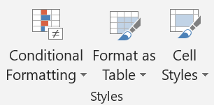
Conditional Formatting…in the Home tab.
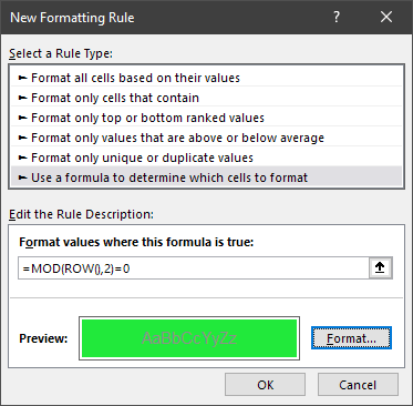
- You will be presented with a pop-up window called New Formatting Rule. Under the Select a Rule Type section, click
Use a formula to determine which cells to format. - Then in the Edit the Rule Description: section, under the Format values where this formula is true: enter the following formula
=MOD(ROW(),2)=0.
- Select
Format...to open the Format Cells window. Here you can select the text color, background color, font type, size, style and etc. to format the cells the way you would like to differentiate the rows. - Once you specify your formatting, select
OK. You will be back to the New Formatting Rule window. Here you will notice a small Preview section to view how your formatted rows would look like. - If you are happy with the formatting settings, select
OK, and there you have it folks! A never ending alternating row colors for your data!
How it Works
As you can see, coloring alternate rows or just alternating the colors on every other row is fairly simple. If you do use the Conditional Formatting route to implement this, here is an explanation on how that works. I always imagine the Conditional Formatting to be these magical fairy bots that are ready and eager to do some colorful work for you and all it needs are some instructions before they go do it.
Let’s Split it Up
The modulo function =MOD() takes in two parameters: the number, and the divisor. In my attempt to avoid talking about a lot of math, it is just another fancy term for the remainder after a division has occured between two numbers. For example, when you divide 5 by 2, you are left with a quotient of 4 (2 x 2 = 4) and a remainder of 1 (5 – 4 = 1). In the case of the =MOD() function, we want to focus on that remainder number. When you divide 4 by 2 on the other hand, you are left with a quotient of 2 (2 x 2 = 4) and a remainder of 0 (4 – 4 = 0). Table 1 goes into more detail on the quotient and remainder you get if you were to enter =MOD(x,2) where x is 0 to 10.
The row function =ROW() just returns a row number of the reference, in our case, the “current” row since the conditional formatting steps through each row to apply the formatting.
This is a clever technique when you use the modulo function and your divisor is 2 – it is a quick and easy way to identify whether a number is even or odd. If it is odd, the =MOD() will return 1, if it is even, the =MOD() will return 0.
| NUMBER (OR CURRENT ROW) | DIVISOR | QUOTIENT | REMAINDER |
|---|---|---|---|
| 1 | 2 | 0 | 1 |
| 2 | 2 | 1 | 0 |
| 3 | 2 | 1 | 1 |
| 4 | 2 | 2 | 0 |
| 5 | 2 | 2 | 1 |
| 6 | 2 | 3 | 0 |
| 7 | 2 | 3 | 1 |
| 8 | 2 | 4 | 0 |
| 9 | 2 | 4 | 1 |
| 10 | 2 | 5 | 0 |
And Put it Together
When you enter a custom formula in the Conditional Formatting you are essentially telling the program “If this formula is true, apply the colors” – hence the name Conditional Formatting!
When you put these two pieces together =MOD() and =ROW() you will get either a 0 or a 1. You run that through the condition of the conditional formatting and you say that if the modulo (or remainder) of the current row is even, then apply the color. Otherwise the little fairy bots will ignore the row and leave it empty.
This is a post about how to alternate the colors of rows in Excel. To learn it in Google Sheets, click here


