When you are working with a lot of data, often times you find the need to visually be able to distinguish it between rows. Beyond the pleasing aesthetics, alternating row colors also allow you to follow the relevant data down the row without losing your place by making it more legible. There are 2 viable ways to alternate row colors in Google Sheets.

As always, you can use some sample data to follow along if you wish. Simply follow the link below to take you to the Google Sheets worksheet then select File > Make a Copy

Using a Table

As of the publish date of this post, Google Sheets doesn’t have the capability of creating a table as it is possible within Microsoft Excel.

Using the Explore Feature or Alternating Colors

Google Sheets or as a matter of fact, most of the G Suite apps have a nifty Explore feature on the bottom right indicated by either an arrow that looks like or in Google Sheets . This is a quicker way to set your data to alternate color between rows. To do so:

Select a cell within your data
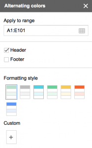
Click on the Explore button on the bottom-right side of the window. This will open a sidebar to edit the formatting. You can also access this by selecting Format from the top menu and selecting Alternating Colors...

Figure 1: Google Sheets Explore Sidebar Alternate Section

Under the section FORMATTING you can select one of the preset colors, or you can select Edit for additional customization
If you select Edit, here you will get a chance to indicate whether you have a header or footer to your data by selecting either the Header or the Footer options

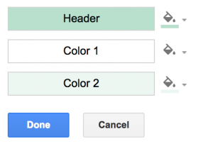
Figure 2: Google Sheets Alternate Colors Edit Header Footer

You can select a custom color, indicate the Header, Color 1, and Color 2 options to set your odd or even row colors.
Once you have made your picks, select Done

Figure 3: Google Sheets Alternate Colors Edit

Conditional Formatting

Highlight the range you would like to format. Alternatively, you can press CTRL + A on Windows or CMD + A on Mac to select the range of filled data
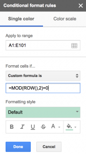
Click Format > Conditional Formatting… This will open a sidebar with options to apply conditional formatting to your data

Figure 4: Google Sheets Conditional Format Rules Sidebar

Under the section Format cells if… click on the dropdown and select Custom formula is
Then in the text box below, enter the following formula:
=MOD(ROW(),2)=0
Under the section Formatting style, you can select a color, and text formatting
Select Done

Note: Using the Conditional Formatting method will yield a truly alternating colored rows without a separate header row. You will need to separately and manually highlight and color the header row.

How it Works

As you can see, coloring alternate rows or just alternating the colors on every other row is fairly simple. If you do use the Conditional Formatting route to implement this, here is an explanation on how that works. I always imagine the Conditional Formatting to be these magical fairy bots that are ready and eager to do some colorful work for you and all it needs are some instructions before they go do it.

Let’s Split it Up

The modulo function =MOD() takes in two parameters: the number, and the divisor. In my attempt to avoid talking about a lot of math, it is just another fancy term for the remainder after a division has occured between two numbers. For example, when you divide 5 by 2, you are left with a quotient of 4 (2 x 2 = 4) and a remainder of 1 (5 – 4 = 1). In the case of the =MOD() function, we want to focus on that remainder number. When you divide 4 by 2 on the other hand, you are left with a quotient of 2 (2 x 2 = 4) and a remainder of 0 (4 – 4 = 0). Table 1 goes into more detail on the quotient and remainder you get if you were to enter =MOD(x,2) where x is 0 to 10.

The row function =ROW() just returns a row number of the reference, in our case, the “current” row since the conditional formatting steps through each row to apply the formatting.

This is a clever technique when you use the modulo function and your divisor is 2 – it is a quick and easy way to identify whether a number is even or odd. If it is odd, the =MOD() will return 1, if it is even, the =MOD() will return 0.

NUMBER (OR CURRENT ROW)	DIVISOR	QUOTIENT	REMAINDER
1	2	0	1
2	2	1	0
3	2	1	1
4	2	2	0
5	2	2	1
6	2	3	0
7	2	3	1
8	2	4	0
9	2	4	1
10	2	5	0

Table 1: =MOD() returns for the first 10 rows

And Put it Together

When you enter a custom formula in the Conditional Formatting you are essentially telling the program “If this formula is true, apply the colors” – hence the name Conditional Formatting!

When you put these two pieces together =MOD() and =ROW() you will get either a 0 or a 1. You run that through the condition of the conditional formatting and you say that if the modulo (or remainder) of the current row is even, then apply the color. Otherwise the little fairy bots will ignore the row and leave it empty.